Sample Jump Model, Comparability Ratio Model, and Standard Regression Model Analysis
This example is an analysis of trends in Melanoma of the Skin cancer mortality rates from 2000-2022 from the U.S. Mortality database. It will show how to use the Jump Model, Comparability Ratio Model and Standard Model in Joinpoint. The Jump Model / Comparability Ratio Model in the Joinpoint software provides a direct estimation of trend data (e.g. cancer rates) where there is a systematic scale change, which causes a “jump” in the rates, but is assumed not to affect the underlying trend. For further information on these models, please reference the Jump Model / Comparability Ratio Model help.
Using Joinpoint
There are four basic steps involved in generating any Joinpoint trend analysis. Review the description of the process:
- Creating an Input Data File for Joinpoint (or for this exercise you can use the file below created for this exercise)
- Setting Parameters in the Joinpoint Program
- Executing the Joinpoint Regression Program
- Viewing the Joinpoint Results
Then walk through the example, Running a Jump Model, Comparability Ratio Model and Standard Regression Model Analysis in Joinpoint, using files created for this purpose.
Creating an Input Data File for Joinpoint
The Joinpoint input file must be an ASCII text file or Excel spreadsheet. Refer to the Joinpoint help system for details concerning the format of this file. You may use SAS, SPSS, Excel, Word, or any software package to create the text file. For the example, we have used the SEER*Stat program to create a text input data file. SEER*Stat provides a convenient mechanism for generating the statistics, exporting the statistics to a text file, and providing the file format information required by Joinpoint.
The input data file for this example was created by exporting SEER*Stat results. SEER*Stat created two files when exporting data:
- Sample.Jump.CR.Standard.Data.txt is the data exported from SEER*Stat. You will use this file as the Input Data File for this exercise.
- Sample.Jump.CR.Standard.Dictionary.dic is the SEER*Stat dictionary file that accompanies the exported txt file.
Setting Parameters in the Joinpoint Program
The Joinpoint Regression Program requires that you specify parameters that are organized on three tabs: the Input File tab, the Method and Parameters tab, and the Advanced Analysis Tools tab.
Input File Tab
The Input File tab specifies the file format of the input data file and some additional settings for the model. For this exercise, the default settings were used for the:
- By Variables
- Dependent Variable
- Independent Variable
- Log Transformation
- Autocorrelated errors options
- Heteroscedastic Errors Option
- Shift data points by
- Include/Exclude Select Cohorts
Joinpoint is able to determine the settings for these based on the information in the SEER*Stat dictionary. If your input data file did not come from SEER*Stat, you would need to set the appropriate values for these controls.
Method and Parameters Tab
The Method and Parameters tab specifies the:
- Modeling method
- Constraints on the location(s) of the joinpoints
- Number of joinpoints
- Model selection method
- AAPC ranges and confidence interval methods
Most parameters on this tab will be set to default values. Joinpoint will try to set the appropriate maximum number of joinpoints by scanning the input data file and locating the cohort with the most observations. Joinpoint will then set the maximum by using the table documented in the Number of Joinpoints help section.
Advanced Analysis Tools Tab
The Advanced Analysis Tools tab can be used to set up these advanced options:
- Pairwise Comparison
- Jump Model/Comparability Ratio
The Pairwise Comparison is only relevant if you have a By Variable defined on the Input File tab. The Jump Model/Comparability Ratio is explained more in this example. There will also be enhancements to this tab in the future that include multi-group clustering.
Executing the Joinpoint Regression Program
Once an input data file has been created and loaded into the session, and parameters have been selected, the program can be executed by clicking the green execute button on the Joinpoint toolbar. A progress meter will be shown on the screen while the Joinpoint calculation engine processes the data and generates the output. Note, it can take a few minutes to execute, depending on the size of the input data file and the options selected. After execution has completed, Joinpoint opens an output window to display the results.
View the Joinpoint Results
Method and ParametersFor standard Joinpoint analyses, the output window displays the results on five tabs: Graph, Data, Model Estimates, Trends, and Model Selection. When using the Pairwise Comparison or Jump Model options, an additional tab labeled with the appropriate option will be shown. There is a cohort tree located to the left of the tabs to traverse the cohorts and various joinpoints in your analysis.
The results of your session are not automatically saved. If you close the output window without saving your results, you will need to re-run the analysis. The results can be saved to a Joinpoint output file (i.e. Sample.Jump.CR.Standard.Output.jpo) by selecting Save or Save As from the File menu, or by clicking on the Save button on the toolbar. The results can be sent to a printer, PDF, Word, or Excel by clicking the Print button from the Joinpoint toolbar, and there are options to customize which elements of the output to include. The results can also be exported as text files and image files (for the graphs) by clicking the Export button on the toolbar making your selections.
Running a Jump Model, Comparability Ratio Model and Standard Regression Model Analysis in Joinpoint
- Download the following files to use in this exercise by right clicking on the link and using Save Link As... to save the file on your computer:
- Sample.Jump.CR.Standard.Dictionary.dic is the SEER*Stat export dictionary used in this exercise. It contains the information describing the layout of the export data file. You will use this file to set up your session specifications.
- Sample.Jump.CR.Standard.Data.txt is the data exported from SEER*Stat. You will use this file as the Input Data File for this exercise.
If you have the SEER*Stat software, you may open or download the SEER*Stat matrix file Sample.Jump.CR.Standard.SEERStat.Results.sim. Please note that you can only access the US Mortality data by running SEER*Stat in client-server mode. For specifics on how to access the US Mortality data using SEER*Stat, please go here.
The rates and confidence intervals were exported to a text file (Sample.Jump.CR.Standard.Data.txt) using the SEER*Stat export feature. View the SEER*Stat export dictionary (Sample.Jump.CR.Standard.Dictionary.dic) for more information regarding the contents of the sample input file. - Open Joinpoint and click the New button from the toolbar. The Open file dialog will open.
- Browse to the folder where you saved the files for the exercise and open the Sample.Jump.CR.Standard.Dictionary.dic file.
- The Joinpoint Session will open to the Input File tab with the following fields filled in:
- Input Data File - Sample.Jump.CR.Standard.Data.txt
- The first 20 records from the Sample.Jump.CR.Standard.Data.txt file will be displayed
- Dependent Variable - Run Type – Provided in Data File
- Type of Variable - Age-Adjusted Rate
- Age-Adjusted Rate - Age-Adjusted Rate
- Standard Error - Standard Error
- Independent Variable –Year of Death (1992-2014)
- Shift data points by - 0
- Interval Type - Annual
- Heteroscedastic Errors Option - Standard Error (Provided)
- By Variables - none
- Log Transformation - Yes {ln(y) = xb}

- Go to the Advanced Analysis Tools tab.
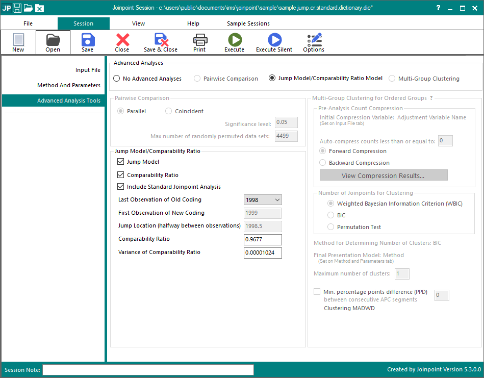
On this tab you will set the appropriate Jump Model and Comparability Ratio parameter values. Please do the following:- In the Advanced Analysis options box, please select the Jump Model/Comparability Ratio Model option.
Both the Jump Model and Comparability Ratio Model require you to know when the scale changed occurred (e.g. when the last year of ICD-9 was used). The Jump Model / Comparability Ratio Model in the Joinpoint software provides a direct estimation of trend data (e.g. cancer rates) where there is a systematic scale change, which causes a “jump” in the rates, but is assumed not to affect the underlying trend. This scale change is usually due to a change in the way the data is coded. Because of this, you need to supply the location of the last data point before the coding change occurs. The software automatically locates the discontinuity or “jump” halfway between this last data point and the next one. The software currently only allows for a single “jump”. For example, the ICD code changes (reference: Anderson et al. 2001) from ICD-9 to ICD-10 for classification rules for selecting underlying causes of death. The last year that ICD-9 was used was 1998, and ICD-10 was implemented starting in 1999. If the user had entered annual data, they would enter 1998, and the software would place the “jump” at 1998.5. For the Comparability Ratio Model, in addition to where the last observation of the old coding is, you need to supply two additional parameter values:- The comparability ratio
- The variance of the comparability ratio
For this exercise, most default settings were used. The following settings need to be changed:- Jump Model/Comparability Ratio:
- Check all three options:
- Jump Model
- Comparability Ratio
- Include Standard Joinpoint Analysis
- Set the “Last Observation of Old Coding” to 1998.
- Once the previous parameter is set, Joinpoint will automatically set the “First Observation of New Coding” to 1999 and the “Jump Location (halfway between observations)” to 1998.5. You cannot override these 2 values.
- Set the “Comparability Ratio” to 0.9677
- Set the “Variance of Comparability Ratio” to 0.00001024
- Check all three options:
- All the session parameters have now been set. Click on the Execute button on the toolbar to execute the session. The progress dialog opens showing the progress of the Joinpoint software. When it is complete, the Output Results opens with the Graph tab displayed.
- To save the results so that they can be opened up later in Joinpoint without re-running the analysis, click the Save button and choose an appropriate file name and location. Please note that when you save the results, you also save the session parameters with it. Once a results file is open, you can retrieve the session that was used to produce it by using the Retrieve Session button on the Joinpoint toolbar. There is no need to save BOTH the session and output results to file.
- To export the results as text files, click the Export button on the Joinpoint toolbar. The Export dialog will open.
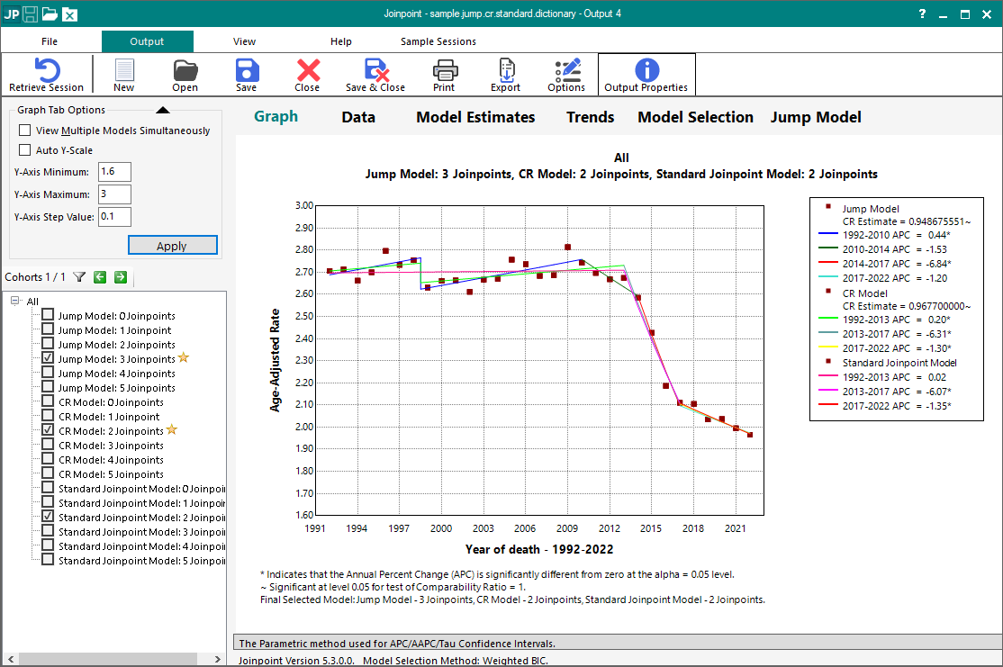
The following graph is the result of the session in the example for a maximum of 4 joinpoints. It is a graph of the age-adjusted melanoma of the skin mortality rates from the US Mortality data, for all races, both sexes from 1992 to 2014. The following models are drawn on the graph:
- Jump Model
The Jump Model is two line segments joined at a joinpoint at 2009. The model increases until 2009, then decreases to 2014. You’ll notice a large drop in the first line segment at 1998.5. This is the location of the Jump Point. - Comparability Ratio Model
The Comparability Ratio Model is two line segments joined at a joinpoint at 2010. The model increases until 2010, then decreases to 2014. You’ll notice a large drop in the first line segment at 1998.5. Again, this is the location of the Jump Point. - Standard Joinpoint Model
In this case, the model is two line segments joined at 2010. There is no Jump Point in a Standard Joinpoint Model.
The APCs (Annual Percent Change) indicate the magnitude of the trend for each model segment or time period.
This example is an analysis of trends in melanoma of the skin age-adjusted mortality rates from 1992-2014 in the United States. The input data file used contains age-adjusted mortality rates and standard errors by year of death. We used the SEER*Stat software to generate these rates for melanoma of the skin in the 9 SEER registries, 1992-2014.