An official website of the United States government

Sample CanSurv Analysis
In this example, we analyze the survival data by historic stage, i.e., localized, regional and distant, for the colorectal cancer patients who are diagnosed during 1973-2001 in the SEER nine cancer registries. The data were exported from SEER*Stat.
There are four steps involved in CanSurv analysis. As you review the description of each step in this exercise, you may view or download the files that were created in the process.
Step 1: Create an Input Data File for CanSurv
Step 2: Set Parameters in the CanSurv Program
Step 3: Execute the CanSurv Program
Step 4: View the CanSurv Results
Step 1: Create an Input Data File for CanSurv
Currently, CanSurv can only accept the input data created by a SEER*Stat survival session. To create a new SEER*Stat survival session select New from the File menu, and then choose Survival session. The default is grouped survival data. To create a case-listing of survival data, select Case Listing from the Session menu. See the SEER*Stat help for information about survival sessions.
Because CanSurv models the net survival due to cancer, only choose the relative survival or cause-specific survival on the Statistic tab in a SEER*Stat Survival session. The Selection tab is used to select the records to be included in the analysis and the Table tab is used to determine which variables are used to stratify the results. The Parameters tab in a Survival session specifies the dates, intervals, and vital status involved with the calculation of survival time. The default options on the Parameters tab are Cumulative summary table, Number of Intervals=60, and Months Per Interval=1. In order to create the survival data for CanSurv, uncheck Cumulative summary and check Standard life table. Although CanSurv can analyze monthly data, the computation is slower than yearly data. To speed up the calculation, set Months Per Interval=12 and change the Number of intervals accordingly.
Once a result matrix is created, it can be exported to a text (*.txt) data file. The associated information about the variable names, format, and the name and location of the data file is saved in the dictionary (*.dic) file. CanSurv uses the information in the dictionary file to read the data file.
The input file for this example contains grouped relative survival data by historic stage for the colorectal cancer patients who are diagnosed in 1975-2015. If you have the SEER*Stat software, you may open or download CanSurvSample_Colorectal.ssm, the SEER*Stat matrix file. The survival data, which include historic stage and life table and expected survival, were exported to a text file (CanSurvSample_Colorectal.txt) using the SEER*Stat export feature. View the SEER*Stat export dictionary (CanSurvSample_Colorectal.dic) for more information regarding the contents of the sample input file.
Step 2: Set Parameters in the CanSurv Program
The CanSurv web app allows users to specify the model and output options directly online.
Input File
If the input file was extracted from SEER*Stat, a dictionary file (*.dic) and a data file (*.txt) were created. The SEER*Stat dictionary file and data file should be stored under the same directory. By default, “SEER*Stat Dictionary and Data Files” is selected under Input Type. Use the Choose Files button to choose the correct location and name of the data files. Note: Since the data file is linked to the dictionary file by its name, it cannot be opened if it has been renamed. Download the following files to use in this exercise:
- CanSurvSample_Colorectal.dic - this is the SEER*Stat export dictionary to use in this exercise, and
- CanSurvSample_Colorectal.txt - this is the data exported from SEER*Stat. This will be used as the Input Data File.
The other Input Type is the “Workspace” option, which can load the results of a previous CanSurv analysis.
After selecting the correct data files, CanSurv will automatically output the Data Type contained in the data (e.g., Relative Survival in Proportions).
The Model Specifications section allows users to select the specific model to be fit. CanSurv can fit standard parametric survival models, Cox PH models, and mixture cure models. The default for standard survival models is the Cox proportional hazards model, and the default latency distribution G(t) for the cure models is the lognormal distribution. If a mixture cure model is to be fit, the “Cure in Model” option should be selected. Possible distributions for parametric survival modeling include the Lognormal (the default distribution), Loglogistic, Weibull, or Gompertz. Users can also select a Semiparametric model, which fits a Cox proportional hazards model. In this exercise, a mixture cure model with a lognormal distribution was fitted.
Next, users specify the Computation Specifications. These specifications control the parameters of the Newton-Raphson algorithm and are autopopulated with default values. Unless the user has prior experience with running CanSurv models, it is recommended to leave the default values as is. In this exercise, the default computation specifications were used.
The Analysis Variables portion of the Model Specifications tab autopopulates with variables read in from the SEER*Stat.dic and .txt files. Users have options to select whether the variable is categorical or continuous, whether the variable is a stratum variable, and whether the variable should be included in the modeling of µ, σ, or the cure parameter. In this exercise, SEER historic stage A was used as a categorical variable, and it was used in µ and cure for the mixture cure model.
The final Notifications section allows for users to enter their email address if the analysis to be run may be computationally intensive. In this case, users will receive an email with a link to the results once the job is completed.
Step 3: Execute the CanSurv Program
Click Submit once all data and model specifications have been made.
Step 4: View the CanSurv Results
A window with four tabs will pop up after the calculation finishes. The Report tab summarizes the model parameters and likelihood, and in this example, returns, the cure fractions for the analysis variable stage. Users have the option to display more decimal places for improved accuracy.
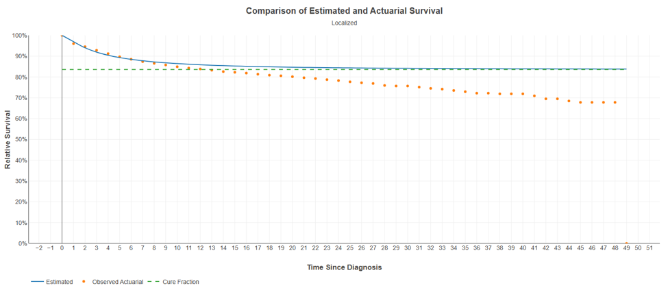
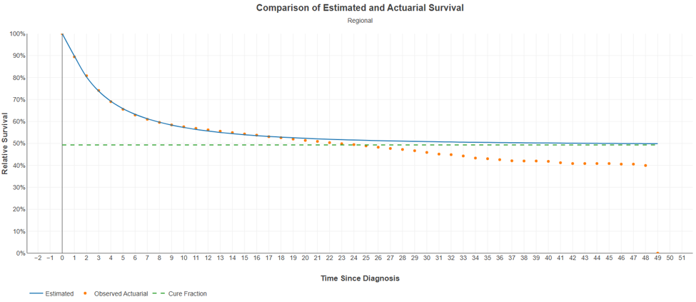
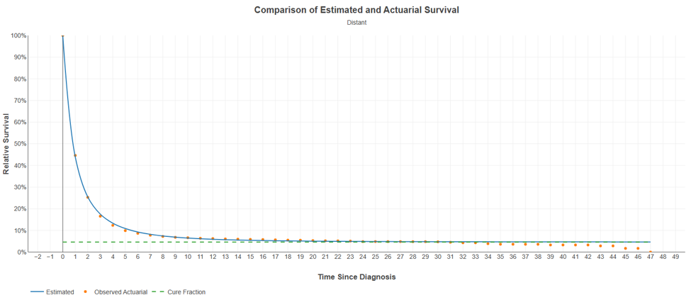
The Estimated and Actuarial Survival Curves tab shows the estimated survival, observed actuarial survival, and cure fraction for a given cohort by time since diagnosis. The K-Year Survival Rate tab shows the estimated and observed actuarial K-year survival by the analysis variable. The Deviance Residuals tab plots deviance residuals by time since diagnosis. The LogLikelihood L(c) vs c plot tab displays the loglikelihood as a function of the cure fraction, and it is only available if no covariates are used in the cure fraction estimation. Because stage is included as a cure variable in this example, this plot is not produced.
In each tab containing plots, users have the option to copy or save the plot. In addition, the data used to produce each plot are included as a table and can be downloaded.
The following graphs were created by CanSurv when the mixture cure model with lognormal latency distribution was executed. These are scatter plots of the actuarial and relative survival curves for localized, regional, and distant stage colorectal cancer.
Users can save the entire CanSurv session by selecting the Export Workspace option in the upper righthand corner, which saves the results as a .zip file.