Sample Age-Adjusted Rate Calculation and Regression Analysis

This example is an analysis of trends in colorectal cancer incidence rates from 1993-2013 in the SEER cancer registries. It will show you what information is needed to have Joinpoint compute Age-Adjusted rates and how to provide that information to the Joinpoint program.

An age-adjusted rate is a weighted average of crude rates, where the crude rates are calculated for different age groups and the weights are the proportions of persons in the corresponding age groups of a standard population. Age-adjusted rates are usually expressed as the number of cases per 100,000 population at risk. When computing crude rates, Joinpoint allows you to display rates as cases per 1,000; 10,000; 100,000; or 1,000,000. For the age-adjusted rate formula, please refer to the SEER*Stat tutorial.

For a detailed explanation on how to set up your data file so Joinpoint can compute age-adjusted rates from it, please reference the following help section: How to Compute Age-Adjusted Rates in Joinpoint.

Using Joinpoint

There are four basic steps involved in generating any Joinpoint trend analysis. Review the description of the process, and then we will walk you through a regression analysis example using files created for this purpose.

1. Creating an Input Data File for Joinpoint (or for this exercise you can use the file below created for this exercise)
2. Setting Parameters in the Joinpoint Program
3. Executing the Joinpoint Regression Program
4. Viewing the Joinpoint Results

---

Creating an Input Data File for Joinpoint

The Joinpoint input file must be an ASCII text file. Refer to the Joinpoint help system for details concerning the format of this text file. You may use SAS, SPSS, Excel, Word, or any software package to create this text file.

The following input file is provided for this exercise:

• Sample.Age.Adjusted.Rate.Calculation.Data.txt contains the counts, populations, and standard populations for this exercise.

When computing age-adjusted rates, Joinpoint requires the input data file to contain the necessary variables to compute the rates but also to have them in a specific order. Below is a list of the required variable order. Cohort-defining variables are only required when you have more than one cohort in your data file. All other variables in the list are required in order to have Joinpoint compute age-adjusted rates.

• All cohort-defining variables (in this example it is “Sex”)
• Independent variable (in this example it is “Year of diagnosis”)
• Adjustment variable (this is typically an age variable)
• Count
• Population
• Standard Population

Setting Parameters in the Joinpoint Program

The Joinpoint Regression Program requires that you specify parameters that are organized on three tabs: the Input File tab, the Method and Parameters tab, and the Advanced Analysis Tools tab.

Input File Tab

The Input File tab specifies the file format of the input data file and some additional settings for the model. Please refer to the Joinpoint program's online help for more information regarding the options on this tab.

Method and Parameters Tab

The Method and Parameters tab specifies the modeling method, constraints on the location(s) of the joinpoints, number of joinpoints, model selection method, AAPC Segment Ranges, and APC/AAPC/Tau confidence interval methods. For this exercise, the default settings on the Method and Parameters tab tab were used.

Advanced Analysis Tools Tab

The Advanced Analysis Tools tab can be used to set up a parallel or coincident pairwise comparison or a Jump Model/Comparability Ratio Model analysis. The pairwise comparison is only relevant if you have one or more By Variables defined on the Input File tab.

Executing the Joinpoint Regression Program

Once an input data file has been created and loaded into the session, and parameters have been selected, the program can be executed by clicking the green execute button on the Joinpoint toolbar. A progress meter will be shown on the screen while the Joinpoint calculation engine processes the data and generates the output. Note, it can take a few minutes to execute, depending on the size of the input data file and the options selected. After execution has completed, Joinpoint opens an output window to display the results.

Viewing the Joinpoint Results

For standard Joinpoint analyses, the output window displays the results on five tabs: Graph, Data, Model Estimates, Trends, and Model Selection. When using the Pairwise Comparison or Jump Model options, an additional tab labeled with the appropriate option will be shown. There is a cohort tree located to the left of the tabs to traverse the cohorts and various joinpoints in your analysis.

The results of your session are not automatically saved. If you close the output window without saving your results, you will need to re-run the analysis. The results can be saved to a Joinpoint output file (i.e. Sample.Session.jpo) by selecting Save or Save As from the File menu, or by clicking on the Save button on the toolbar. The results can be sent to a printer, PDF, Word, or Excel by clicking the Print button from the Joinpoint toolbar, and there are options to customize which elements of the output to include. The results can also be exported as text files and image files (for the graphs) by clicking the Export button on the toolbar making your selections.

Running an Age-Adjusted Rate Calculation Regression Analysis in Joinpoint

1. Download the following file to use in this exercise by right clicking on the link and using Save Link As... to save the file on your computer:
   • Sample.Age.Adjusted.Rate.Calculation.Data.txt is the data file containing the information needed to compute age-adjusted rates. You will use this file as the Input Data File for this exercise.
     
     The input data file for this example contains incidence counts and associated populations by sex and year of diagnosis.
2. Open Joinpoint and click the New button from the toolbar. The Open file dialog will open.
3. Browse to the folder where you saved the files for the exercise and open the Sample.Age.Adjusted.Rate.Calculation.Data.txt file.
4. The Joinpoint session window will open and will automatically have the Input File tab displayed. Below is a picture of the window you should see.
   
   
   
   The following options at the top of the screen should be automatically filled in:
   • Column headers - checked
   • Delimiters – Tab
   • Missing Characters - Space
   • Thousands Separator – Comma
   • Decimal Separator - Period
   Joinpoint will display the first twenty records of the input file. Below the input file viewer are the controls that you need to fill in. Because you want Joinpoint to calculate age-adjusted rates, please set the following options:
   • Run Type: Calculated From Data File option
   • In the Type box please select Age-Adjusted Rate
   • In the Rates Per combo box, please select 100,000
   Once you have made the previous selections, the screen should look like the following:
   
   
   
   Please make the following selections:
   • Count Variable – Select the “Count” variable from the list.
   • Population Variable – select the “Population” variable from the list.
   • Adjustment Variable – select the “Age Group” variable from the list.
   • Standard Population – select the “Standard Population” variable from the list.
   • Log Transformation – Yes {ln(y) = xb}
   • Independent Variable - select the “Year of Diagnosis” variable from the list.
   • Shift data points by - 0
   • Heteroscedastic Errors Option - Standard Error (Calculated)
   • Choose an errors model to fit - Uncorrelated
   • By Variables – click the “Add…” button, select the “Sex” variable, and click Ok. You should see the “Sex” variable in the By Variables list.
5. The last item that needs to be addressed on the Input File tab is to format the values of the Sex variable. The Sex variable has numeric values from 0 to 2 in the data file. Joinpoint provides the ability to display a text string in the output results for each numeric value of the By Variables. If you do not provide a format label for each value, then the numeric value will appear in the output. To have the output be more legible, we want to display labels (e.g. “Male and Female”, “Male”, and “Female”) instead of numbers. In order to build a format for the sex variable, first click on the Sex variable in By Variables box (once you do that the variable name will be highlighted). Then click on the “Define…” button located on the lower right-hand corner of the By Variables box. The “Edit Format” window will appear.
   
   Format labels must be entered as “value = label” in the format box at the bottom of the window. Please enter the following three “value=label” entries in the box.
   0=Male and Female
   1=Male
   2=Female
   The format screen should look like this when you are finished:
   
   
   
   Once you have entered the “value=Label” entries, click on the Ok button.
   
   The Input File Tab of your Session should now look like this:
   
   
6. All the parameters on the Method and Parameters tab and Advanced Analysis Tools Tab will default to the correct settings. So, there is nothing to adjust on either tab.
7. Click on the Execute button on the toolbar to execute the session. The progress dialog opens showing the progress of the Joinpoint software. When it is complete, the Output Results opens with the Graph tab displayed.
8. To save the results so that they can be opened up later in Joinpoint without re-running the analysis, click the Save button and choose an appropriate file name and location. Please note that when you save the results, you also save the session parameters with it. Once a results file is open, you can retrieve the session that was used to produce it by using the Retrieve Session button on the Joinpoint toolbar. There is no need to save BOTH the session and output results to file.
9. To export the results as text files, click the Export button on the Joinpoint toolbar. The Export dialog will open.

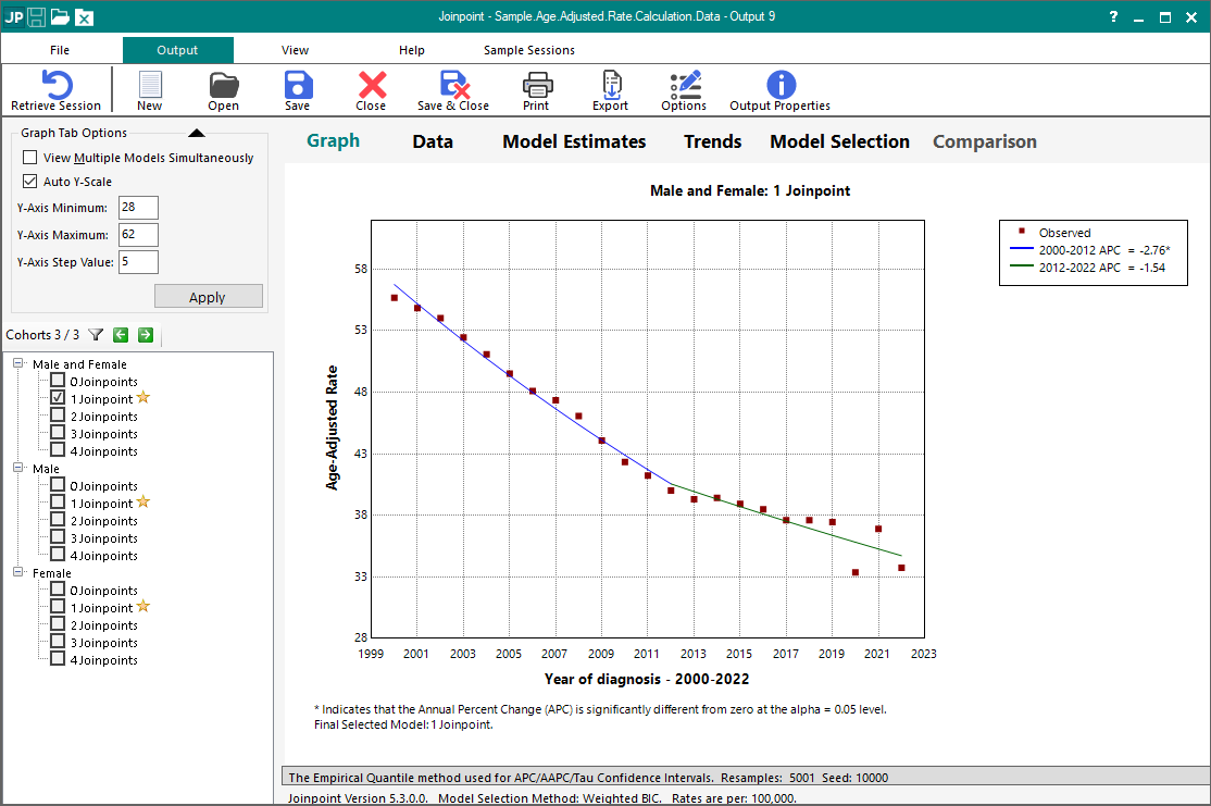
The following graph is the result of the session in the example for a maximum of 3 joinpoints. It is a scatter plot of the age-adjusted colorectal cancer incidence from SEER, for males and females from 1993 to 2013. A Joinpoint Model is also drawn on this graph. In this case, the model is four line segments joined at the joinpoints of 1995, 1998, and 2008. The model decreases until 1995, it increases again until 1998, decreases until 2008 and then decreases more until 2013. The APCs (Annual Percent Change) indicate the magnitude of the trend for each segment or time period.

This example is an analysis of trends in colorectal cancer age-adjusted incidence rates from 1993-2013 in the SEER cancer registries. The input data file used contains counts, populations, and standard populations which Joinpoint used to produce age-adjusted incidence rates and standard errors by year of diagnosis and sex. We used the SEER*Stat software to generate the input data file for this example.